In this post, we will explain how to create a Pivot Table in Google Sheets. A pivot table is a powerful statistical tool that allows you to summarise or aggregate smaller sets of data based on an extensive database. It helps you analyze new relationships and connections between various data sets, by giving you a more focused view of the database. It also allows you to shift (pivot) the table’s axis and see the details of your data from a different angle.

If you’re new to pivot tables and want to learn how to create a pivot table in Google Sheets, then you’ve come to the right place. In this post, we will show you how to create and use a pivot table to filter information as per your need. Let’s get started.

How to create a Pivot Table in Google Sheets?

Google Sheets allows you to create a pivot table for some raw data that you’ve already entered into the spreadsheet. You can group data manually or automatically, and then move the fields to derive useful insights from your data. By changing the way the data is presented, you may easily and quickly compare large quantities of data.

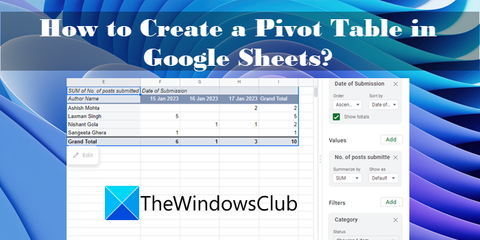
The basic requirement of creating a pivot table is that you must have a raw database that’s been organized in columns within a worksheet, with each column having its own header. For example, take a look at the above image. We have created a database wherein we show the number of blog posts submitted by authors of TheWindowsClub from different categories on different dates. Now we will show you how to create a date-wise distribution of the total number of posts submitted in each of the categories using pivot tables.

Select the data range. For the above example, we have selected the entire database, you may select a portion of data as per your requirement. Go to Insert > Pivot table.

In the Create pivot table dialogue box, specify where you’d like to insert the pivot table, and then click on the Create button. You can insert it in the existing worksheet or in a new worksheet. If you choose to insert it in the same worksheet, you’ll have to specify the location (cell) from where the pivot table should start building. 

When you do this, a blank table will appear. Along with it, a Pivot table editor will appear on the right side of the spreadsheet. At the top of the editor is a ‘Suggested‘ section. Look if any of the suggested pivot tables will help with your query. If it does, you can simply do a mouse click, and Google Sheets will automatically create a base pivot table for you. Otherwise, you will have to manually choose the ‘Rows’, ‘Columns’, ‘Values’, and/or ‘Filters’ to create your pivot table. These are basically various dimensions from which you may analyze your data.

Click on the Add button next to the Rows option. You will see a list of all column headings from your source table. Click on one of the headings to mark the column’s unique values as the row headings of your pivot table. 

Next, click on the Add button next to the Columns option. You will again, see the list of column headings from your source table. Choose one heading to mark the column’s unique values as the column headings of your pivot table. 

The ‘Rows’ and ‘Columns’ will make a two-dimensional dataset for you. Based on these dimensions, you may create a third dimension (Values) to fill your pivot table. Click on the Add button next to the Values option and select another column heading. Now you may apply a function (SUM, AVERAGE, MAX, PRODUCT, COUNT, etc.) to summarize the data of this particular column.  

Last, you may apply a Filter (optional) to further drill down your data to a specific subset. Filters are based either on data values or on conditions (such as is empty, is less than, text contains, date is after, is not equal to, etc.)

Notes:

• You may show/hide the totals of your Rows and Columns values.
• You may display your Rows and Columns data in ascending or descending order.
• You may also sort your Rows or Columns data based on different parameters.
• Changes you make to the pivot table will reflect in real-time.

Read: How to automatically generate Charts and Graphs in Google Sheets.

Using a Pivot Table in Google Sheets

You may use a pivot table to answer questions or build reports required by your boss or supervisors. 

Let us say the boss wants to know how many articles have been submitted by each author from the ‘Windows’ category. To answer this, we have applied a filter on our pivot table. First, we clicked on the Add button next to the Filters option. Then we selected the ‘Category’ option. From the Status dropdown, we unchecked all other items except for ‘Windows’. 

As we clicked on OK, the pivot table showed just the data we required!

This is how to create and use a pivot table in Google Sheets. Hope you find this useful.

Read Next: How to create a Pivot Table and Pivot Chart in Excel.