Microsoft Excel is a powerful tool widely used for data analysis, management, and reporting. One of its essential features is the ability to work with dates and perform various operations involving date-based data. However, there is a common issue that users of Excel encounter when working with date data; that is, Excel does not recognize dates correctly on their computer. In this article, we will learn how to resolve this issue.

Why won’t Excel recognize dates?

Excel does not recognize dates because they are not formatted perfectly. Hereinafter, we have mentioned all the methods by which you can format the date. Once you do that, there won’t be any issues.

Fix Excel not recognizing Dates

If Microsoft Excel does not recognize dates, follow the solutions mentioned below.

1. Format using Text to columns
2. Use the VALUE Function
3. Deploy The DATEVALUE Function
4. Replace unsupported delimiters

Let’s get started.

1] Format using Text To Columns

The Text to Columns functionality divides text contained within a solitary column into multiple columns using a designated delimiter, such as a comma or space. This even holds true for dates formatted as text, maintaining a consistent delimiter.
Upon utilizing the Text to Columns function, Excel can identify a date that was formerly stored as text and subsequently transform it into a recognizable date layout.

Pick any cell within your date column and examine the formula bar. Should you spot an apostrophe preceding the date character, it indicates that the date has been formatted as. However, if the date column is left-aligned instead of right, it is formatted as text.

Once you’ve confirmed that your dates are formatted as text, you can employ the Text to Columns tool to make things right. To do this, follow the prescribed steps:

•  Pick the column that holds the date data which are not recognized.
• Navigate to Data (Excel Ribbon) > Text to Columns.
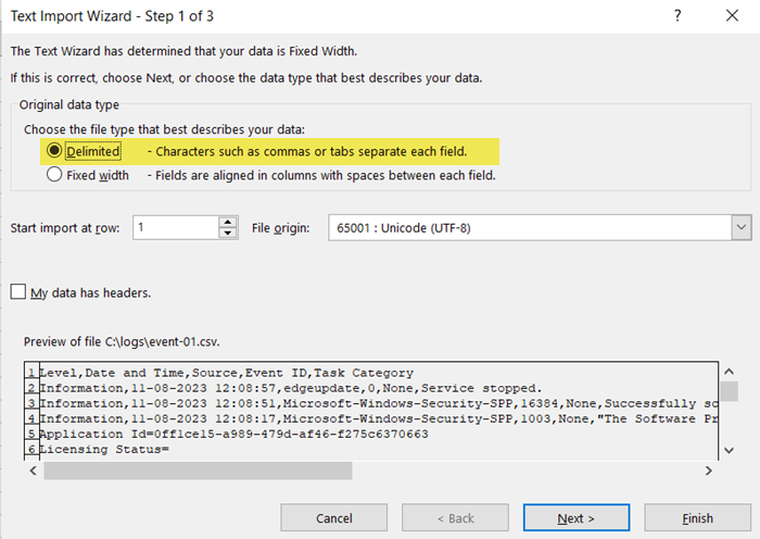
• Within the Text to Columns Wizard dialog box, choose the Delimited alternative and proceed by clicking Next.
• Select the desired delimiter from the available options to separate your data. Use the Other option to enter the appropriate delimiter if it’s unavailable on the list.
• Pick the column containing the date information and choose the Date option under Column data format. Select the date format that matches the format of the date that you have entered.
• Choose the remaining columns that hold the time portion of the data and under Column data format, select the option Do not import column (skip). This way additional columns will not be exported.
• Upon completion, proceed by clicking the Finish button.

Once these steps are finalized, Excel will appropriately format the data, which you can then use for further calculations and analysis.

It’s important to be aware that this approach might not always be effective, particularly in cases where the date data is input in an unconventional format; that’s why, move to the next solution.

Read: How to Insert and Calculate Formulas and Functions in Excel?

2] Use the VALUE Function

If the Text to Columns feature fails to perform, consider utilizing the VALUE function as an excellent substitute. This alternative is particularly advantageous in scenarios where date values are intertwined within extensive text strings or lack uniform formatting, posing challenges for the Text to Columns tool to precisely divide the date values.

The VALUE function performs the task of transforming numeric text into actual numerical values, extracting these values from a text string, including date values represented as text. This proves especially beneficial in situations where a uniform delimiter fails to consistently divide the date values, or when the format varies within the text string.

Utilizing the VALUE function is a straightforward process, as it requires just a single argument, which is the text itself. With this, you only need to reference the cell containing the date Excel doesn’t recognize.

Follow the prescribed steps to use the VALUE function to solve the said error:

• Input the formula =VALUE(A2) into a cell that is currently vacant.
• This action will result in the conversion of the date information stored in cell A2 into a serial number which Excel uses to create dates.
• Highlight the cell that contains the serial number and go to the Number section in the Home menu ribbon.
• Click General and select the Short Date option.

By following this process, the serial number will be transformed into a date format, and hopefully, the issue will be resolved.

Note: Replace A2 with the exact number of the cell that depends on its coordinates. So, for example, if the date is in Column B and starts from the second row, you need to enter B2.

Read: How to compare two columns in Excel using VLOOKUP?

3] Deploy the DATEVALUE Function

The DATEVALUE function operates in a similar manner to the VALUE function but the difference is that it automatically generates the output in a date format, whereas the VALUE function simply returns the serial number of the date.

DATEVALUE has only one function date_text, which is also very similar to the text argument in the VALUE function.

So, if Excel does not recognize the date format, using the DATEVALUE function, just enter the formula =DATEVALUE(A1) in the formula field and refer to the cell containing the date that Excel fails to recognize.

Note: Replace A1 with the number of the cell. So, for example, if the date is in Column B and starts from the second row, you need to enter B2.

Make sure that the date is not in the format of your system time. For example, if your system format is DD/MM/YYYY, the date can be DD-MM-YYY or some other format.

Also Read: How to lock cells in Excel formula to protect them?

4] Replace unsupported delimiters

We can find all the unsupported delimiters and replace them with the ones you use. For example, if the delimiter, in your case, is ‘/’, if you accidentally put ‘.’ instead, that cell will not have the right format. That is why, we must maintain consistency. To find the black sheep, we have a perfect feature called Find and Replace. Follow the steps mentioned below to deploy it.

• Open Microsoft Excel.
• Press the Ctrl +H key to open the Find and Replace option.
• Enter the delimiter that is causing inconsistency in the Find what field.
• In the Replace with field, enter the delimiter with which you want to replace the inconsistent one with.
• Then, proceed to click the “Replace All” button.

Once you click the Replace All, Excel will execute the modifications, while also providing you with a count of the total replacements performed. Changing the delimiter alone is sufficient to reformat the dates, which were previously presented as text, into their proper date format.

Hopefully, your issue will be resolved now.

Also Read: Excel not auto calculating formulas

How do you get Excel to recognize a cell as a date?

By default, Excel takes our input as text. That is why, when you want to give a date as an input, you need to format it correctly. There are various methods to do the same. We have mentioned all of them earlier in this post. Just go through them and resolve your issue.

Read: Excel formula not dividing correctly.