In this post, we will show you how to count colored cells in Microsoft Excel.

While working with Excel, we often color-code cells to distinguish them from the rest of the data. This is good because the only concern is to grab someone’s attention. But when we color-code cells to indicate some value (for example, ‘green’ for approved and ‘red’ for not approved), we may require counting these values at some later point in time.

Excel offers plenty of functions, but sadly, none of them can be used directly to calculate the count of color-coded cells. Also, there’s no built-in way (whatsoever) to do so in Excel. However, there are workarounds to count colored cells in Microsoft Excel, which we will discuss in this post. So keep reading!

How to count Colored Cells in Excel?

To count colored cells in Microsoft Excel, you may use the Find and Select tool or the Excel Filter and SUBTOTAL() function. Let us see both these methods in detail.

1] Use the Find and Select tool

The Find & Select tool is used to find and select cells that meet specific requirements. It lets you execute the Find command, Find and Replace command, and Go To commands in Excel. With the help of the Find command, you can count the number of cells that have a specific background color. Here’s how:

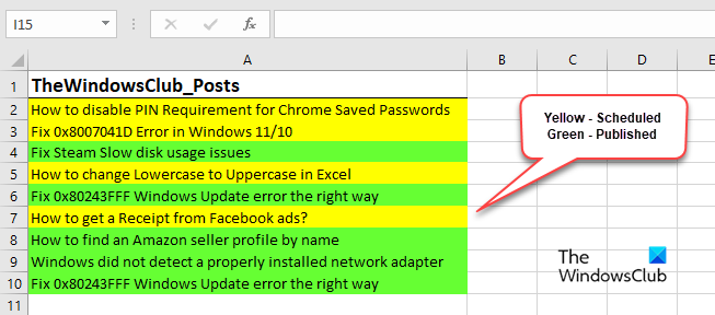
Let’s say we have a worksheet wherein we have some sample data as shown in the above image. The data lists some blog posts that have either been scheduled or published on TheWindowsClub. Here, yellow color has been used to indicate that a post is scheduled, and green color has been used to indicate that a post is published. For this data, we can count the total number of scheduled posts as follows:

Select the data range (A2:A6). Click on the Find & Select dropdown in the Editing section (top right corner). Click on the Find option.

The Find and Replace dialogue box will appear. Click on the Options>> button to expand the dialogue box.

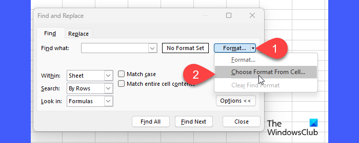
Do not enter anything in the Find what field. Click on the dropdown arrow on the Format button and select the Choose Format From Cell… option.

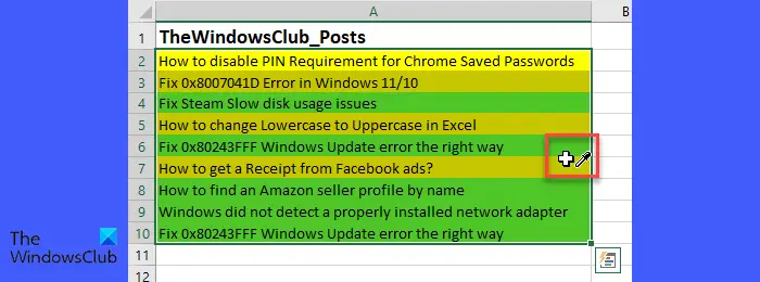
As you select the option, the Find and Replace dialogue box will disappear and your mouse pointer will turn into a plus symbol with a color picker next to it.

Note: If you click on the Format button instead of the dropdown arrow, the Find Format window will appear. You may then click on the Choose Format From Cell button at the bottom of the window to bring out the color picker.

Now take the color picker over a yellow-colored cell and click on it.

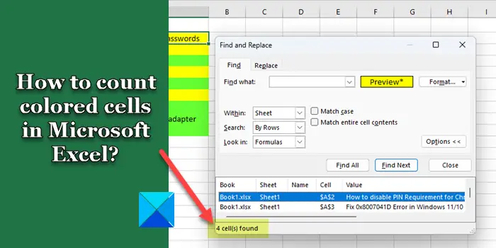
The Find and Replace dialogue box will reappear (if disappeared) and show the selected color in the Preview box. Click on the Find All button at the bottom.

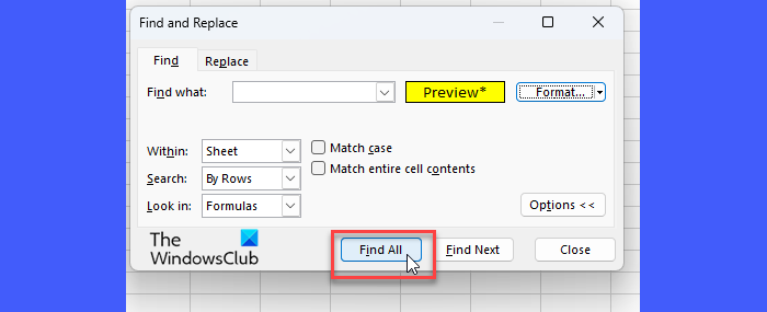
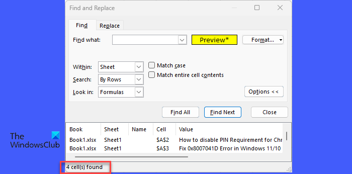
The dialogue box will further expand and show the list of cells that are color-coded in yellow. At the bottom of the dialogue box, you will see the count of these cells.

2] Use Excel Filter and SUBTOTAL() function

The SUBTOTAL() function can be used to perform a calculation on a given range of cells. It can be used to apply other functions on the cell range while ignoring the cells that shouldn’t be part of the calculation. A total of 11 functions are supported by the SUBTOTAL() function.

It has the following syntax:

SUBTOTAL(function_num,ref1,[ref2],...)

Where,

• function_num  is the numeric reference to the function that should be used in the calculation. It takes either 1 to 11 or 101 to 111 as value. For example, 1 or 101 for AVERAGE(), 2 or 102 for COUNT(), 3 or 103 for COUNTA(), etc. The variation in the numeric reference determines whether to include(1-11) or exclude(101-111) hidden cell values in the function.
• ref1 refers to the cell range whose subtotal is required.
• ref2 refers to another cell range for the calculation. This may go up to ref254.

Taking the same example as above, we can count the total number of scheduled posts using the SUBTOTAL() function as follow:

Place your cursor in cell A11 and type the following function in the Formula Bar on top:

=SUBTOTAL(103,A2:A10)

Here, value ‘103’ indicates that the COUNTA() function has been referred to in the SUBTOTAL() function. Also, it indicates that hidden values will be excluded, if any. If you have numeric data in your worksheet, you may refer to the COUNT() function (2/102).

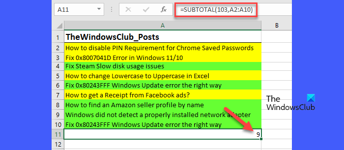
Since there are no hidden rows at this moment, the count comes out to be 9. When you manually hide rows with green cells, the SUBTOTAL() function automatically shows the updated results (8, 7, etc.).

If the data is quite large (which is obvious), manually hiding rows could be tedious. So you can add a filter to show only yellow-colored cells in the data range.

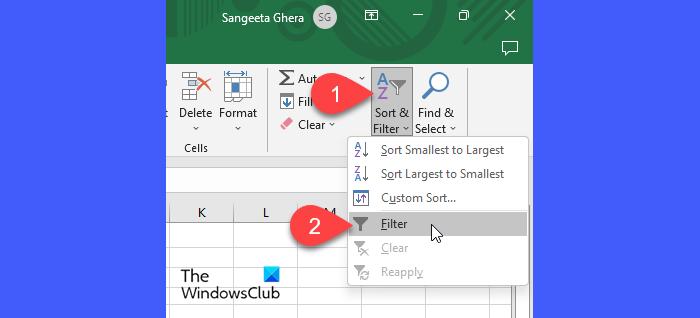
Click on the Sort & Filter tool just before the Find & Select tool. Select the Filter option from the dropdown.

A down arrow icon will appear in each column header. Click on that icon and select Filter by Color > Yellow.

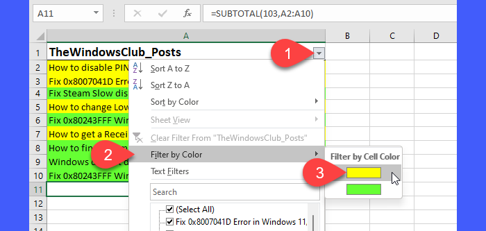
This will filter out yellow-colored cells. The result of the SUBTOTAL() function will also update based on the visible data.

Note: When SUBTOTAL() function is used on filtered data, hidden values are always ignored regardless of the function_num argument.

So this is how you can count colored cells in Microsoft Excel. I hope you find this useful.

Also Read: How to highlight Cell or Row with Checkbox in Excel.

Can Excel count by colored cells?

There’s no built-in way to count colored cells in Excel, but there’s a trick. You can apply a color filter to the cell values and then count only visible cells by passing the COUNT() or COUNTA() function as an argument in the SUBTOTAL() function. The SUBTOTAL() function can be used to perform various arithmetic operations (sum, count, average, etc.) on a given cell range.

Can you use Countif with colors?

COUNTIF() function cannot be used to check the background color, foreground color, or any other formatting in Excel. It is a statistical function that only works with values. If you want to count colored cells in a worksheet, you may use the Find feature. Press Ctrl+F to bring the Find and Replace dialogue box. Click on Format > Choose Format From Cell. Take the pointer-turned-color picker to the colored cell and do a mouse click. Click on the Find All button. The count will be shown at the bottom of the Find and Replace window.

Read Next: How to create a dropdown list with color in Excel and Google Sheets.